반응형
혼동 행렬(Confusion matrix)
혼동 행렬(Confusion matrix)은 분류 문제에서 모델을 학습시킨 뒤, 모델에서 데이터의 X값을 집어넣어 얻은 예상되는 y값과, 실제 데이터의 y값을 비교하여 정확히 분류 되었는지 확인하는 메트릭(metric)이라고 할 수 있습니다.
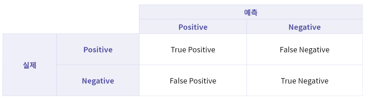
위 표가 바로 혼동 행렬이며, 각 표에 속한 값은 다음을 의미합니다.
- True Positive (TP) : 실제 값은 Positive, 예측된 값도 Positive.
- False Positive (FP) : 실제 값은 Negative, 예측된 값은 Positive.
- False Negative (FN) : 실제 값은 Positive, 예측된 값은 Negative.
- True Negative (TN) : 실제 값은 Negative, 예측된 값도 Negative.
사이킷런 안에는 위 4개 평가 값을 얻기 위해 사용할 수 있는 기능이 정의되어 있습니다.
이번 실습에서는 3개의 클래스를 가진 다중 분류 데이터를 이용하여 혼동 행렬을 직접 출력해보고,확인해보도록 하겠습니다.
혼동 행렬을 위한 사이킷런 함수/라이브러리
- from sklearn.metrics import confusion_matrix : 혼동 행렬(Confusion matrix) 을 위한 기능을 불러옵니다.
- confusion_matrix(y_true, y_pred)
: Confusion matrix의 값을 np.ndarray로 반환해줍니다.
from elice_utils import EliceUtils
elice_utils = EliceUtils()
import warnings
warnings.filterwarnings(action='ignore')
import numpy as np
import matplotlib.pyplot as plt
from sklearn.svm import SVC
from sklearn.datasets import load_wine
from sklearn.model_selection import train_test_split
from sklearn.metrics import confusion_matrix
from sklearn.utils.multiclass import unique_labels
# 데이터를 불러와 학습용, 테스트용 데이터로 분리하여 반환하는 함수입니다.
def load_data():
X, y = load_wine(return_X_y = True)
class_names = load_wine().target_names
train_X, test_X, train_y, test_y = train_test_split(X, y, test_size =0.3, random_state=0)
return train_X, test_X, train_y, test_y, class_names
# Confusion matrix 시각화를 위한 함수입니다.
def plot_confusion_matrix(cm, y_true, y_pred, classes, normalize=False, cmap=plt.cm.OrRd):
title = ""
if normalize:
title = 'Normalized confusion matrix'
else:
title = 'Confusion matrix'
classes = classes[unique_labels(y_true, y_pred)]
if normalize:
# 정규화 할 때는 모든 값을 더해서 합이 1이 되도록 각 데이터를 스케일링 합니다.
cm = cm.astype('float') / cm.sum(axis=1)[:, np.newaxis]
print(title, ":\n", cm)
fig, ax = plt.subplots()
im = ax.imshow(cm, interpolation='nearest', cmap=cmap)
ax.figure.colorbar(im, ax=ax)
ax.set(xticks=np.arange(cm.shape[1]),
yticks=np.arange(cm.shape[0]),
xticklabels=classes, yticklabels=classes,
title=title,
ylabel='True label',
xlabel='Predicted label')
# label을 45도 회전해서 보여주도록 변경
plt.setp(ax.get_xticklabels(), rotation=45, ha="right",
rotation_mode="anchor")
# confusion matrix 실제 값 뿌리기
fmt = '.2f' if normalize else 'd'
thresh = cm.max() / 2.
for i in range(cm.shape[0]):
for j in range(cm.shape[1]):
ax.text(j, i, format(cm[i, j], fmt),
ha="center", va="center",
color="white" if cm[i, j] > thresh else "black")
fig.tight_layout()
plt.savefig('confusion matrix.png')
elice_utils.send_image('confusion matrix.png')
"""
1. 혼동 행렬을 계산하고,
시각화하기 위한 main() 함수를 완성합니다.
Step01. 데이터를 불러옵니다.
Step02. 분류 예측 결과를 평가하기 위한 혼동 행렬을 계산합니다.
Step03. confusion matrix를 시각화하여 출력합니다.
plot_confusion_matrix 함수의 인자를 참고하여
None을 채워보세요.
3-1. 혼동 행렬 시각화 결과를 확인합니다.
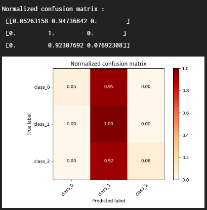
3-2. 함수의 인자 normalize값을 True로 설정하여
정규화된 혼동 행렬 시각화 결과를 확인합니다.
"""
def main():
train_X, test_X, train_y, test_y, class_names = load_data()
# SVM 모델로 분류기를 생성하고 학습합니다.
classifier = SVC()
y_pred = classifier.fit(train_X, train_y).predict(test_X)
cm = confusion_matrix(test_y, y_pred)
plot_confusion_matrix(cm, test_y, y_pred, classes = class_names)
# 정규화 된 혼동 행렬을 시각화합니다.
plot_confusion_matrix(cm, test_y, y_pred, classes = class_names, normalize = True)
return cm
if __name__ == "__main__":
main()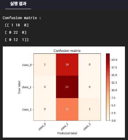

반응형
'AI & 머신러닝 coding skill' 카테고리의 다른 글
| 머신러닝 분류 - 정확도(accuracy), 정밀도(precision), 재현율(recall) (0) | 2022.05.24 |
|---|---|
| 머신러닝 분류 - 사이킷런을 활용한 나이브 베이즈 분류 (0) | 2022.05.24 |
| 머신러닝 분류 - 나이브 베이즈 분류 (0) | 2022.05.24 |
| 머신러닝 분류 - SVM(Support Vector Machine) (0) | 2022.05.24 |
| 머신러닝 Decision tree - 앙상블(Ensemble) 기법 - Bagging (0) | 2022.05.24 |
| 머신러닝 Decision tree - 앙상블(Ensemble) 기법 - Voting (0) | 2022.05.24 |
| 머신러닝 의사결정 나무(DecisionTree Classifier) - 분류 (0) | 2022.05.24 |
| 머신러닝 의사결정 나무(DecisionTree Regressor) - 회귀 (0) | 2022.05.24 |


